False-positive brain: Do you really have to correct for multiple comparisons in an analysis of variance?

If your stats class was anything like mine, you learned that using ANOVA instead of  t-tests is a sneaky way to avoid the multiple testing problem. I still believed this until very recently and a lot of my colleagues are bewildered, when I try to convince them otherwise. Of course this has been covered quite a bit. For example, there is an awesome blog-post by Dorothy Bishop and there is this great recent paper . In addition to that, today, I want to share a simple way to convince yourself this truly is a problem using some simulated data and SPSS.

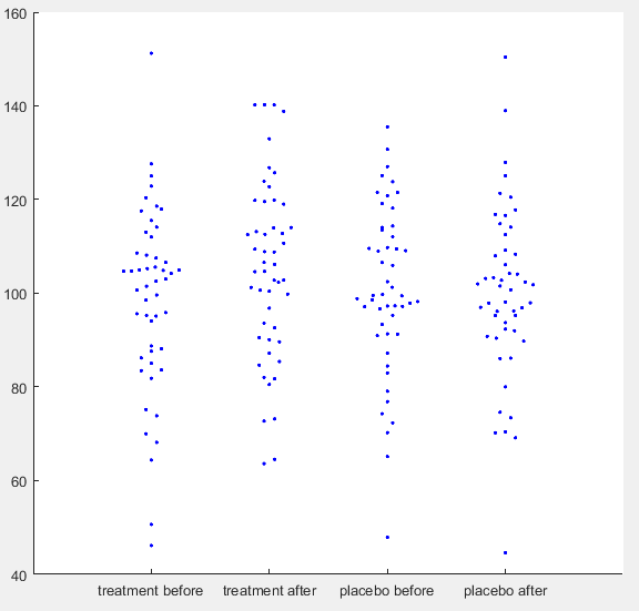
Simulated IQ-data. First a ground truth was simulated with mean = 100 and SD = 15 for 50 participants. For each condition normally distributed noise was added with mean = 0 and SD = 8. For ‘treatment after’ additionally a normally distributed effect was added with mean = 5 and SD = 10. (See MATLAB code for details)

Let’s say you have run a simple experiment on intelligence, where you wanted to find out, if a drug enhances problem solving capacity. You ran two experimental days, one day you gave placebo the other day you gave the treatment. On each experimental day you first ran your IQ-test for a baseline measurement and then gave the participant either the treatment or a placebo. When the drug was ingested you tested IQ again, assuming that an increase would happen only in the treatment condition. After running 50 participants, you get the data plotted above. You open SPSS and run a repeated measures ANOVA defining your first factor as a treatment factor with the levels treatment vs. placebo and your second factor as a time point factor with the levels before vs. after. In your output below you find no significant main effect of treatment (p = 0.246), no main effect of time point (p = 0.062), but as you predicted there is an interaction between treatment and time point (p = 0.026). You publish this in Science and get tenure.

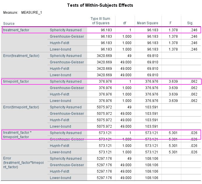
Data analysed in SPSS 24 using the GLM command (see SPSS script for details).

However, there is an alternate way of getting p-values for these data. Instead of running a repeated measures ANOVA you can do some addition or subtraction to get rid of one factor and then use repeated measures t-tests to compare the remaining conditions. For example, to analyse a treatment effect you add the before and after values from the treatment and the placebo condition, respectively, and compare them. Which works similarly for the time point effect. For the interaction you have to deduct the before condition from the after condition for both treatment conditions and then compare. Below is the output of this approach and it may surprise you that you get exactly the same p-values (0.246, 0.062, 0.026) as from the ANOVA. If you Bonferroni correct these none of them remain significant.

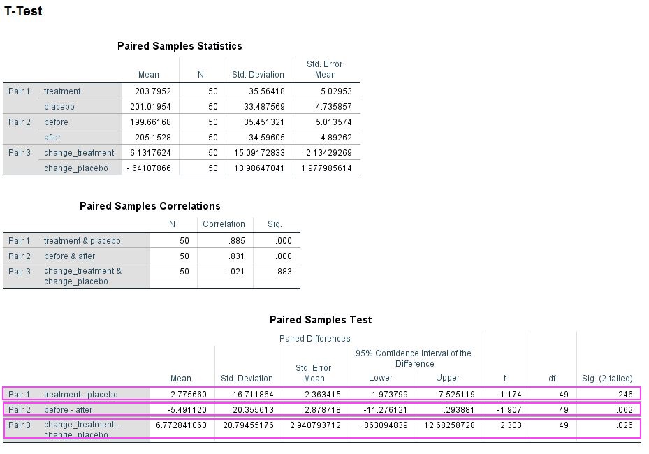
Data summed and analysed in SPSS 24 using the TTEST command (see SPSS script for details).

For me this approach was an eye-opener, as in your first stats lesson you learn that running three t-tests means you must correct for multiple comparisons. Since you get the same p-values running ANOVA, it obviously does not magically self-correct for this problem and you have to manually correct as for t-tests. I have added my simulated data and my SPSS-script so you can try this out yourself (you can also check out my MATLAB code). Once you have convinced yourself, do also check out the resources in the intro to understand why this is the case. Importantly, this problem goes away, if you preregister the interaction as your effect of interest, but then strictly you must not calculate the main effects. Please let me know, what you think about this little demonstration in the comments.

Download data

MATLAB Code

[codesyntax lang=”matlab”]

clear all
rng(20202222, 'Twister')

%here we set the amount of subjects
subs = 50;

%here we generate some random numbers as ground truth, e.g. IQ
mean_t = 100;
SD_t = 15;
truth = normrnd(mean_t,SD_t,subs,1);

%here we set the measurement error. the higher it is the lower
%retest-reliability
error_variance = 8;

%effect size (ratio of variance and mean is effect size)
effect_variance = 10;
mean_effect = 5;

%Here we generate data from our "Experiment" with 2 repeated measures
%factors, e.g. treatment vs placebo and before vs. after
data(:,1) = truth+normrnd(0,error_variance,subs,1);
data(:,2)= truth+normrnd(0,error_variance,subs,1)...
+normrnd(mean_effect,effect_variance,subs,1);
data(:,3)= truth+normrnd(0,error_variance,subs,1);
data(:,4)= truth+normrnd(0,error_variance,subs,1);

%we sum some of the data for t-tests
data(:,5)=sum(data(:,1:2),2);
data(:,6)=sum(data(:,3:4),2);
data(:,7)=sum(data(:,[1 3]),2);
data(:,8)=sum(data(:,[2 4]),2);
data(:,9)= data(:,2)-data(:,1);
data(:,10)= data(:,4)-data(:,3);
data(:,11)=sum(data(:,1:4),2);

%quick t-test to see if there is a significant difference
[h,p] = ttest(data(:,1),data(:,2));

%here you can check the correlations, you should aim for something
%realistic
reliability = corrcoef(data(:,1:4));

%create variable name header for SPSS
Header = {'before_treatment' 'after_treatment' 'before_placebo' ...
'after_placebo' 'treatment' 'placebo' 'before' 'after' ...
'change_treatment' 'change_placebo' 'all_data'}; %header
textHeader = strjoin(Header, ',');

%write header to file
filename = 'ANOVA_blog_data.csv';
fid = fopen(filename,'w');
fprintf(fid,'%s\n',textHeader)
fclose(fid)

%write data to end of file
dlmwrite(filename,data,'-append');

[/codesyntax]

SPSS syntax

PRESERVE.
SET DECIMAL DOT.

GET DATA  /TYPE=TXT
  /FILE="...\ANOVA_blog_data.csv"
  /ENCODING='UTF8'
  /DELIMITERS=","
  /QUALIFIER='"'
  /ARRANGEMENT=DELIMITED
  /FIRSTCASE=2
  /DATATYPEMIN PERCENTAGE=95.0
  /VARIABLES=
  before_treatment AUTO
  after_treatment AUTO
  before_placebo AUTO
  after_placebo AUTO
  treatment AUTO
  placebo AUTO
  before AUTO
  after AUTO
  change_treatment AUTO
  change_placebo AUTO
  @all AUTO
  /MAP.
RESTORE.
CACHE.
EXECUTE.
DATASET NAME DataSet3 WINDOW=FRONT.


GLM before_treatment after_treatment before_placebo after_placebo
  /WSFACTOR=treatment_factor 2 Polynomial timepoint_factor 2 Polynomial 
  /METHOD=SSTYPE(3)
  /CRITERIA=ALPHA(.05)
  /WSDESIGN=treatment_factor timepoint_factor treatment_factor*timepoint_factor.



DATASET ACTIVATE DataSet3.
T-TEST PAIRS=treatment before change_treatment WITH placebo after change_placebo (PAIRED)
  /CRITERIA=CI(.9500)
  /MISSING=ANALYSIS.