
Recently, I started thinking about the chances of finding that one process is involved in two separate functions. If it affects these functions completely independently and they also do not affect each other, it seems intuitive that finding both functions in one experiment is harder than each of them individually. I put this intuition to test in some simple data simulation. (Of course, if you are more maths savvy than me, you can just come up with some equations to solve this. If this is you, please excuse my inferiority and stop reading here.)

Before I start, I want to give you an example of what I mean. In sleep research, a scientist might want to know something about whether a specific sleep stage (or other specified sleep process) influences only declarative, only procedural memory, both or neither. To find out, one might set up an experiment, where one runs two independent tasks that recruit these two memory systems, respectively. One would then manipulate whether the participants stay awake or nap for 60 minutes (such a nap usually only contains slow wave sleep). Assuming that both memory systems benefit equally from slow wave sleep, but are otherwise completely independent, how big are your chances of finding this in these data?
Of course, this depends also partially on your statistical approach. In my experience, many researchers would run their statistics separately on task A and B, as they are assumed to be independent. It would be possible to plug both tasks into a multivariate analysis, but most of the time the research I have seen so far is satisfied to use two univariate analyses. Then the paper would say something along the lines of “task A was significantly affected by our manipulation, whereas task B was not”. Therefore, for sake of argument I will also choose this approach, even though I know that absence of evidence is not evidence of absence.
Concretely in my data simulation (and simulation is clearly overstating what I did, it is really just some simple multiplications) I consider all four possibilities of ground truth (the manipulation is effective for: 1. A and B, 2. only A, 3. only B, 4. Neither). In an experiment, this design can lead to the four corresponding findings (the manipulation is effective for: 1. A and B, 2. only A, 3. only B, 4. Neither), but depending on truth condition a proportion of these will be false or true, all depending on the power and alpha-level set in the experiment. I chose to use the standard alpha-level of 0.05, since this is quite widely accepted. For power, I used the range from 0.05 to 0.95 to see how it affected the results and set both tasks to always have equivalent power. You can see the data in the figure below.
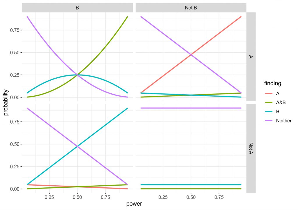
Three of the four the panels are completely intuitive, but I will give you a quick run through anyway. The bottom right shows the values when the ground truth is that neither A nor B is affected by the manipulation. Obviously, irrespective of the power we correctly reject an effect for both outcomes ~90% of times, whereas for both outcomes individually there is a roughly 5% chance of a false positive (the lines are completely overlapping). Finding that A and B are affected is very unlikely, as you would have to get two false positives simultaneously (0.05 x 0.05). The top right and bottom left are identical, just that either A or B being affected are true. What can be seen here is that the intuitive approach to use independent statistics actually works quite well, the higher the power the higher the chance of getting a hit, but incorrectly finding that B is affected or that both A and B are affected is relatively uncommon.
The top left panel for me is the most interesting. Here, the truth condition is that both A and B are affected by the manipulation. However, at low power there is actually a higher chance that you will find that only A or only B are affected. Also, don’t be fooled by the A&B line being higher after a power of 0.5, since the only A and only B lines are overlapping, it actually takes until a power of ~0.7 until chances are higher to find A and B than either of these. In fact, at a power of 0.5 you have a chance of finding either A or B half of the time, while there is only a chance of 0.25 of finding A and B. Although this is all only simple multiplication and it is intuitive that finding two effects is harder than finding one, the magnitude of the problem was not clear to me. (Importantly, the maths depend on the tasks being independent, as soon as dependence comes in, the results may be very different. In addition, you may find that different tasks have different amounts of noise or the effects are of different size, so power could also be different.)
What does this mean for the research example above? In sleep research, we are often dealing with samples that are on the small side, so we might be running quite low powered studies. This means that when we find that slow wave sleep only affects a declarative task, but not a procedural task, there is the possibility that this is due to the considerations laid out here rather than distinct memory processing. Possibly, one partial solution would be to run multivariate tests or to run a superiority or equivalence test on the data and I might do some simulations on that in future. However, I do think that these data suggest another big problem with running underpowered research. Especially, in research areas, where replication is hardly ever performed and thus such errors can remain undetected.
Let me know, what you think about this. Also happy about resources, if this has been delt with before (likely with more depth). Here is the R code, so you can go and play around, if you want. Full disclosure: I am new to R so I coded this up in Matlab first and then repeated it in R…you can imagine which took longer.
#Here we set up the range of power values we use
power_values <- seq(from = 0.05,to = 0.95, by = 0.01)
#This is our alpha that can be varied, if you want to see what happens
alpha_is <- 0.05
#This sets up an array of NaNs to populate later
outcome_probs <- array(rep(NaN, 4*4*length(power_values)), dim=c(4, 4, length(power_values)))


#This runs a loop for each power value
for (k in 1:length(power_values)) {
     #the kth power value is used
     power_is <- power_values[k]
     #temporary power and alpha are loaded into these vectors
     probsA <- c(power_is, power_is, alpha_is, alpha_is)
     probsB <- c(power_is, alpha_is, power_is, alpha_is)

     #this runs a loop for the 4 different truth conditions
     for (i in 1:4) {
       probA = probsA[i]
       probB = probsB[i]

       #saves the data in the array
       outcome_probs[,i,k] = c(probA*probB, probA*(1-probB), (1-probA)*probB, (1-probA)*(1-probB))
     }

}


#creates a temporary vector to reshape the data
 temp_outcome_probs = matrix(outcome_probs,nrow = 16*length(power_values), byrow = TRUE)
 #turns the data into a data.frame
 outcome_probs_long_df <- data.frame(temp_outcome_probs)
 #adds the column name "probability"
 colnames(outcome_probs_long_df) <- c("probability")

 #adds the variable power values to the data.frame
 outcome_probs_long_df$power <- rep(power_values,each=16)
 #adds the variable finding with the 4 finding conditions
 outcome_probs_long_df$finding <- rep(c("A&B", "A", "B", "Neither"), times = length(power_values)*4)
 #adds the variable truthA with the two truth conditions for A
 outcome_probs_long_df$truthA <- rep(c("A", "Not A"), times = length(power_values), each = 8)
 #adds the variable truthB with the two truth conditions for B
 outcome_probs_long_df$truthB <- rep(c("B", "Not B"), times = length(power_values)*2, each = 4)

 outcome_probs_long_df$truthB

 #loads ggplot
 library("ggplot2")

 #makes a graph with the four truth conditions and lines for each of the four findings
 plot_outcome_probs <- ggplot(outcome_probs_long_df, aes(x=power, y = probability)) +
   geom_line(aes(colour = finding , group = finding), size=1) +
   facet_grid(truthA ~truthB)

 plot_outcome_probs + theme_bw()
Update 1: In a few days the first two PhD-students of my group will be starting. One of them Juli Tkotz has come up with two improved versions of my above code, which I am allowed to share here:
library(tidyverse)

# Function for calculating outcome probability
calculate_finding_prob <- function(finding, probA, probB) {
  prob <- rep(NA, length(finding))
  prob[finding == "AB"] <- probA[finding == "AB"] * probB[finding == "AB"]
  prob[finding == "A"] <- probA[finding == "A"] * (1 - probB[finding == "A"])
  prob[finding == "B"] <- (1 - probA[finding == "B"]) * probB[finding == "B"]
  prob[finding == "neither"] <-
    (1 - probA[finding == "neither"]) * (1 - probB[finding == "neither"])

  return(prob)
}

# Range of power values
power_values <- seq(.05, .95, .01)
# Alpha levels to be examined
alpha <- c(.05, .1)
# Possible "truths" and corresponding probA and probB values
truth_probs <- data.frame(truth = c("AB", "A", "B", "neither"),
                          probA = c("power", "power", "alpha", "alpha"),
                          probB = c("power", "alpha", "power", "alpha"),
                          stringsAsFactors = FALSE)
# Possible findings
findings <- c("AB", "A", "B", "neither")

# Combination of each power value, each alpha level, each truth and each finding
combinations <-
  expand.grid(power = power_values, alpha = alpha, truth = truth_probs$truth,
              finding = findings, stringsAsFactors = FALSE)

# Insert probabilities
# When present: power; else: alpha
combinations$probA <-
  ifelse(truth_probs$probA[match(combinations$truth, truth_probs$truth)] == "power",
         combinations$power, combinations$alpha)

combinations$probB <-
  ifelse(truth_probs$probB[match(combinations$truth, truth_probs$truth)] == "power",
         combinations$power, combinations$alpha)

# Calculate probabilities - formula varies as a function of finding
combinations$probability <-
  calculate_finding_prob(combinations$finding, combinations$probA,
                         combinations$probB)

# For alpha = .05
combinations %>%
  filter(alpha == .05) %>%
  ggplot(aes(x = power, y = probability)) +
  geom_line(aes(colour = finding, group = finding), size = 1) +
  facet_wrap(~ truth, nrow = 2) +
  theme(legend.position = "top")

# For alpha = .1
combinations %>%
  filter(alpha == .1) %>%
  ggplot(aes(x = power, y = probability)) +
  geom_line(aes(colour = finding, group = finding), size = 1) +
  facet_wrap(~ truth, nrow = 2) +
  theme(legend.position = "top")
library(tidyverse)

power_values <- seq(.05, .95, .01) # Range of power values
alpha <- c(.05, .1) # Alpha levels
variables <- c("A", "B", "C")

# GENERATE FINDINGS
# For each variable, we can either find the given variable or nothing ("")
findings <- lapply(variables, function(x) c(x, ""))
# All possible combinations
findings <- expand.grid(findings, stringsAsFactors = FALSE)
# Paste together
findings <- apply(findings, 1, function(x) paste0(x, collapse = ""))
# "" should be "neither"
findings <- ifelse(findings == "", "neither", findings)

# All possible combinations of variables being truly observed or not
var_combs <- rep(list(c(TRUE, FALSE)), length(variables))
names(var_combs) <- variables
var_combs <- expand.grid(var_combs)

# All possible combinations of power, alpha levels and possible findings.
to_add <- expand.grid(power = power_values, alpha = alpha, finding = findings)

# Each "truth combination" has to be combined with every power/alpha/finding
# combination. So, we repeat each row in to_add (power/alpha/finding combination
# for every combination (row) in combinations and the other way round. And then
# merge the whole thing.
# ATTENTION! First, we use "each", then, we use "times"!
# (TO DO: There has to be a more elegant vectorised way of doing this)
comb1 <- to_add[rep(seq_len(nrow(to_add)), each = nrow(var_combs)), ]
comb2 <- var_combs[rep(seq_len(nrow(var_combs)), times = nrow(to_add)), ]
combinations <- cbind(comb1, comb2)

# Truth column: What would have been the true finding.
# We use the rows of the columns that contain variable status as index to
# extract the variables whose effects are truly present.
combinations$truth <-
  apply(combinations[variables], 1,
        function(x) paste0(variables[x], collapse = ""))
combinations$truth <-
  ifelse(combinations$truth == "", "neither", combinations$truth)

# Now, each row is uniquely identifiable by a combination of power, alpha,
# finding and truth, so we can safely gather variables into long format.
# Gather will take the column names to gather from the object variables in the
# environment.
combinations_lf <- combinations %>%
  gather(variable, effect_present, variables)

# Proof: Two variables per combination of power, alpha, finding, truth
combinations_lf %>%
  group_by(power, alpha, finding, truth) %>%
  count()

# We create another column if the effect of a given variable has sucessfully
# been detected, i.e. if the given variable is present in the column finding.
combinations_lf$effect_observed <-
  sapply(seq_along(combinations_lf$variable),
         function(x) grepl(combinations_lf$variable[x], combinations_lf$finding[x]))

# Now, we calculate the probability of effect_observed based on the following
# logic:
# If an effect is     present and     observed -> power
# If an effect is     present but not observed -> 1 - power
# If an effect is not present but     observed -> alpha
# If an effect is not present and not observed -> 1 - alpha

# In other words:
# present:  TRUE = power; FALSE = alpha
# observed: TRUE = x;     FALSE = 1 - x

combinations_lf <-
  combinations_lf %>%
  mutate(var_probability = ifelse(effect_present,
                                  power, alpha))

combinations_lf <-
  combinations_lf %>%
  mutate(var_probability = ifelse(effect_observed,
                                  var_probability, 1 - var_probability))

# We calculate the probability of a given finding by multiplying all the
# probabilities of effect_observed for a combination of power, alpha, finding
# and truth.
combinations_lf <- combinations_lf %>%
  group_by(power, alpha, finding, truth) %>%
  mutate(finding_probability = prod(var_probability))

# Plot for alpha = .05
combinations_lf %>%
  filter(alpha == .05) %>%
  ggplot(aes(x = power, y = finding_probability, colour = finding)) +
  geom_line(size = 1) +
  labs(y = "probability") +
  facet_wrap(~truth) +
  theme(legend.position = "top")

# Plot for alpha = .1
combinations_lf %>%
  filter(alpha == .1) %>%
  ggplot(aes(x = power, y = finding_probability, colour = finding)) +
  geom_line(size = 1) +
  labs(y = "probability") +
  facet_wrap(~truth) +
  theme(legend.position = "top")

