
If one thing has changed my view of stats in the last couple of years, it has been using simulation to explore how they pan out for 10.000 studies.
Using simulation is an approach that Daniël Lakens uses a lot in his free online course on stats. If you haven’t had a look at it yet, I highly recommend you do! This approach makes sense, especially for the NHST approach, since, as Daniel puts it, the α-level mainly prevents you from being wrong too often in the long run. Simulations help you get an intuition what that means. Recently, we prepared a preprint that describes how equivalence tests can be used for fMRI research and while I was preparing Figure 1 for that, I had some insights about effect sizes and the uncertainty of point estimates that seemed worth a blog post.
My background is in biological psychology and cognitive neuroscience, a field that suffers from studies that have small samples and are likely underpowered. Excuses for not changing these habits that I have heard frequently are “effect sizes are large in our field” and “small effects don’t matter”. The former will be the subject of the current post, but hopefully I will also get to write about the latter. Connoisseurs of the replication crisis literature will of course know that, e.g., the effect sizes in fMRI research are inflated by small sample sizes (e.g., Button et al. 2013). This makes sense as the sample size determines the critical effect size that is needed to reach statistical significance. This problem is ameliorated when one reports confidence intervals around the point estimates of effect sizes. Today I want to give an intuition how point estimates of empirical effect sizes behave at different sample sizes, when there is no underlying effect. This gave me a better understanding of what the confidence interval means. Of course, all this will be completely clear to the more mathematically minded without using simulations. However, if you are like me, a visualization will make it much easier to understand.
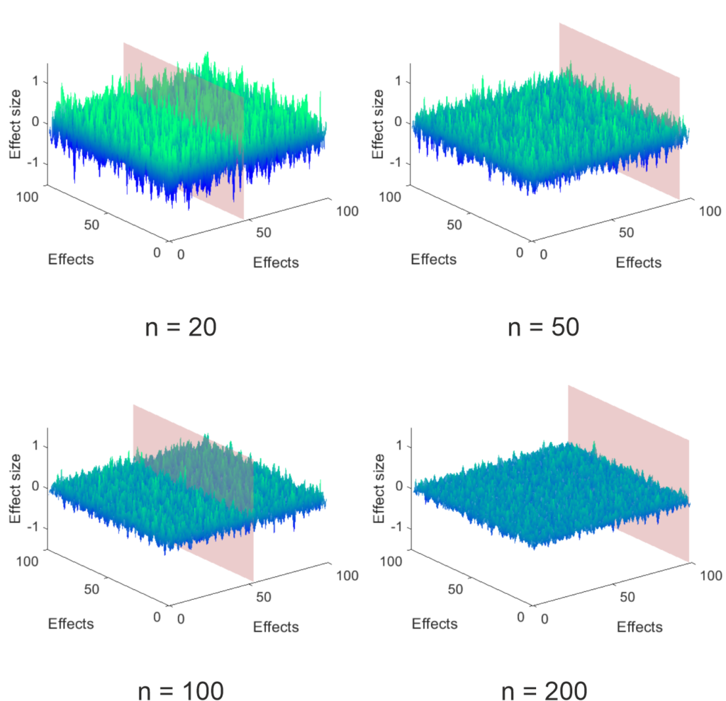
The simulations I performed are very simple. I created a 100 x 100 matrix of simulated experiments (effects) for a control group and an experimental group by picking normally distributed random numbers with a mean of 0 and a standard deviation of 1. I arbitrarily picked the population to be 1000 per group and then randomly selected subsamples to look at the effect of different sample sizes. For each of the 100 x 100 experiments I calculated the effect size (Hedge’s g), which can be seen below, using the MES toolbox by Hentschke and Stüttgen (an awesome resource, if you are using Matlab like me). As you can see at small sample sizes the surface is very rough – a storm on the sea of uncertainty – and gets more and more even as the sample size increases.
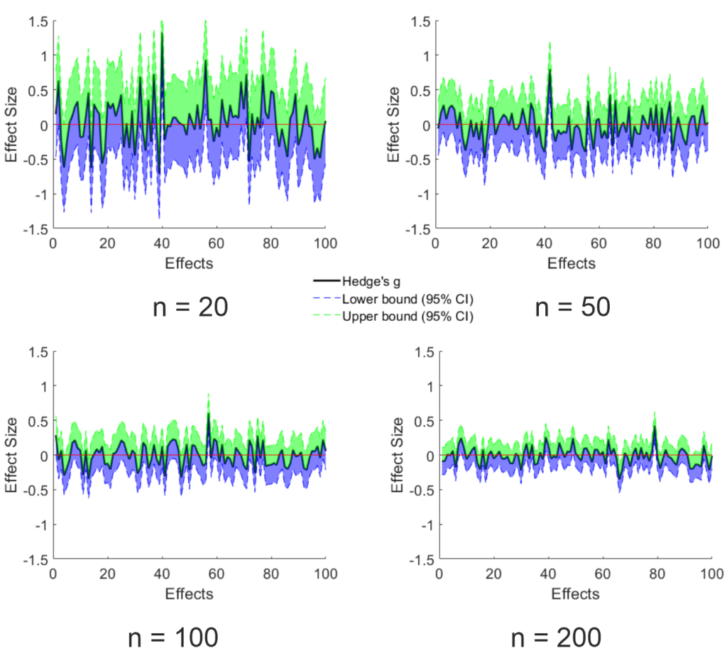
This influence of sample size makes sense since the uncertainty of the point estimate is reduced the larger the sample gets, as can be seen below. For these graphs, I took the data that lies on the plain shown in the above figure (this was set to appear at the largest effect size estimate) and added the 95% CI of the point estimate calculated using the toolbox mentioned above. Trivially, the width of the CI is reduced by increasing sample size. Importantly, since the ground truth is known (I only simulated null effects), the amount of expected false positives remains the same (5%). Since the uncertainty is reduced by sample size, the effect size of the false positives is on average lower the larger the sample is. Something that makes sense, but which I did not expect. I think, this strongly contradicts the “effect sizes are large in our field” argument.
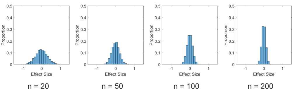
To emphasize this, I also plotted histograms of the effect sizes in this simulation below. As you can see, the effect sizes nicely follow a normal distribution. However, the distribution is much wider for small samples than for large samples. This has to be the case, as on average 5% of the estimated effects must be above (or below for two sided tests) the critical effect size to produce the expected false positives.
As I said above, all of this follows from the math used for NHST, but for me it was a revelation to see the simulations. Of course, so far I have only showed the case, where the null hypothesis is true. I would say nobody thinks we live in a world, where this is always the case. In the next post, I want to look at what happens, when I also simulate true effects. So stay tuned.

